DATABASE MANAGEMENT SYSTEM

Authors

🧑‍💻 RK ROY & Senju Nikhil

🧾 "Databases aren't just about data—they're about trust, speed, and reliability."

Download Full Notes PDF

📚 Data

Data is a collection of raw, unorganized facts and details like numbers, text, images, and more.

• Data is measured in terms of bits and bytes
• Data can be recorded and does not have any meaning unless processed

Types of Data

Quantitative data

• Numerical form
• Examples: weight, volume, temperature

Qualitative data

• Descriptive, but not numerical
• Examples: gender, ethnicity, religion

Information

Provides context of the data and enables decision making.

Database

Database is an electronic place/system where data is stored in a way that it can be easily accessed, managed, and updated. To make real use of data, we need Database Management Systems (DBMS).

DBMS

A DBMS (Database Management System) is software that interacts with users, applications, and the database itself to store, manage, and retrieve data efficiently and securely.

Advantages:

• Data Integrity and Consistency: Ensures accuracy and consistency of data across the database
• Data Sharing: Multiple users and applications can access the database simultaneously
• Data Security: Allows different users to have different levels of access

---

DBMS Architecture

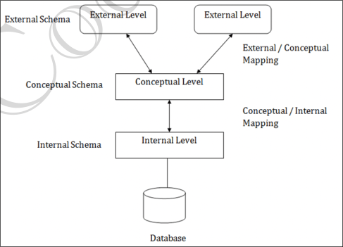
View of Data (Three Schema Architecture)

The purpose is to hide unnecessary details from users and make databases easier to use through three levels of abstraction:

Physical Level (Internal Level)

• Describes how data is actually stored in memory (files, indexes, etc.)
• Deals with low-level data structures, storage allocation, compression, encryption
• Goal: Store data efficiently

Logical Level (Conceptual Level)

• Describes what data is stored and relationships among data
• Users at this level don't worry about physical storage details
• Database designers (DBAs) use this level to plan the database structure
• Goal: Make database easy to design and manage

View Level (External Level)

• Describes how users see the data
• Different users can have different views of the same database
• Uses views/schemas to show only relevant parts of the data
• Also helps secure data by restricting what each user group can see
• Goal: Provide personalized, secure data views

Data Models

Provides a way to describe the design of a DB at logical level. Underlying the structure of the DB is the Data Model; a collection of conceptual tools for describing data, data relationships, data semantics & consistency constraints.

Examples: ER model, Relational Model, object-oriented model, object-relational data model

Database Languages

Data Definition Language (DDL)

• Used to specify the database schema
• We specify consistency constraints, which must be checked every time DB is updated

Data Manipulation Language (DML)

• Used to express database queries and updates
• Data manipulation involves:
  • Retrieval of information stored in DB
  • Insertion of new information into DB
  • Deletion of information from the DB
  • Updating existing information stored in DB
• Query language is a part of DML to specify statements requesting the retrieval of information

Practically, both language features are present in a single DB language, e.g., SQL.

---

Relational Model

Relational Model organizes the data in the form of tables.

Key Concepts:

• Tuple: A single row of the table representing a single data point/unique record
• Degree of table: Number of attributes/columns in a given table/relation
• Cardinality: Total number of tuples in a given relation

Integrity Constraints

Integrity constraints in databases are rules that ensure the accuracy, consistency, and validity of data stored in a relational database. They prevent invalid data from being entered and maintain the logical correctness of relationships among tables.

Domain Integrity

Ensures that values in a column are valid according to the column's data type, range, or format.

age INT CHECK (age >= 0);

Entity Integrity

Ensures that every table has a primary key, and that primary key values are unique and not NULL. Prevents duplicate or missing identifiers for rows.

student_id INT PRIMARY KEY;

Referential Integrity

Ensures consistency between foreign keys and the primary key they reference. Prevents "orphan" records.

FOREIGN KEY (course_id) REFERENCES Course(course_id);

Key Integrity

Guarantees uniqueness of data in certain columns. Includes Primary Key, Unique Key, and Foreign Key constraints.

email VARCHAR(100) UNIQUE;

Check Constraints

Define a condition that each row must satisfy.

salary DECIMAL CHECK (salary > 0);

Relational Model Keys

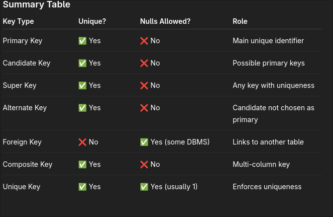
🔑 Simple Key

Key with only one attribute.

🔑 Primary Key

• A column or set of columns that uniquely identifies each row in a table
• Cannot have null values
• There is only one primary key per table
• Example: student_id in student table

🔑 Candidate Key

• Set of all unique keys
• Any column (or combination of columns) that can uniquely identify a row
• A table can have multiple candidate keys, but only one is chosen as the primary key

🔑 Super Key

• Candidate Key ∪ any other attributes
• A set of one or more attributes that can uniquely identify a row
• Candidate key ⊆ Super key
• May contain extra columns

🔑 Alternate Key

• A candidate key that is not chosen as the primary key
• Still uniquely identifies rows

🔑 Foreign Key

• A column in one table that refers to the primary key of another table
• Used to link tables together

🔑 Composite Key

• A key made up of two or more columns that together uniquely identify a row
• Used when a single column is not enough

🔑 Unique Key

• Like a candidate key: ensures all values are unique
• Can allow one null value (depends on DBMS)
• Can be used to enforce uniqueness on non-primary attributes

🔑 Compound Key

• Primary key formed using 2 foreign keys
• Key with more than one attribute

Key Constraints

NOT NULL

Restricts the user from having a NULL value. Ensures every element in the database has a value.

UNIQUE

Ensures that the values in the column are unique.

DEFAULT

Used to set the default value to the column. The default value is added to the columns if no value is specified for them.

CHECK

Keeps the check that integrity of data is maintained before and after the completion of CRUD operations.

PRIMARY KEY

This is an attribute or set of attributes that can uniquely identify each entity in the entity set. Must contain unique as well as not null values.

FOREIGN KEY

Whenever there is some relationship between two entities, there must be some common attribute between them. This common attribute must be the primary key of an entity set and will become the foreign key of another entity set.

---

Entity Relationship Model

Data Models

Collection of conceptual tools for describing data, data relationships, data semantics, and consistency constraints.

ER Model

It is a high level data model based on a perception of a real world that consists of a collection of basic objects, called entities and of relationships among these objects. Graphical representation of ER Model is ER diagram, which acts as a blueprint of DB.

Entity

An Entity is a "thing" or "object" in the real world that is distinguishable from all other objects.

• Entity can be uniquely identified (by a primary attribute, aka Primary Key)
• Strong Entity: Can be uniquely identified
• Weak Entity: Can't be uniquely identified, depends on some other strong entity

Attributes

An entity is represented by a set of attributes. Each entity has a value for each of its attributes. For each attribute, there is a set of permitted values, called the domain, or value set, of that attribute.

Types of Attributes

Simple

• Attributes which can't be divided further
• Example: Customer's account number, Student's Roll number

Composite

• Can be divided into subparts (other attributes)
• Example: Name can be divided into first-name, middle-name, last-name

Single Valued

• Only one value attribute
• Example: Student ID, loan-number

Multi-Valued

• Attribute having more than one value
• Example: phone-number, nominee-name

Derived

• Value can be derived from other related attributes
• Example: Age, loan-age, membership-period

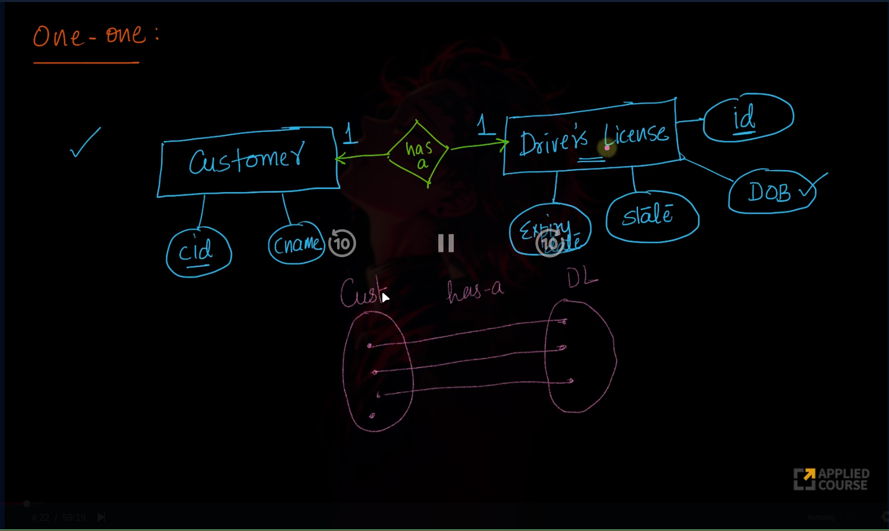
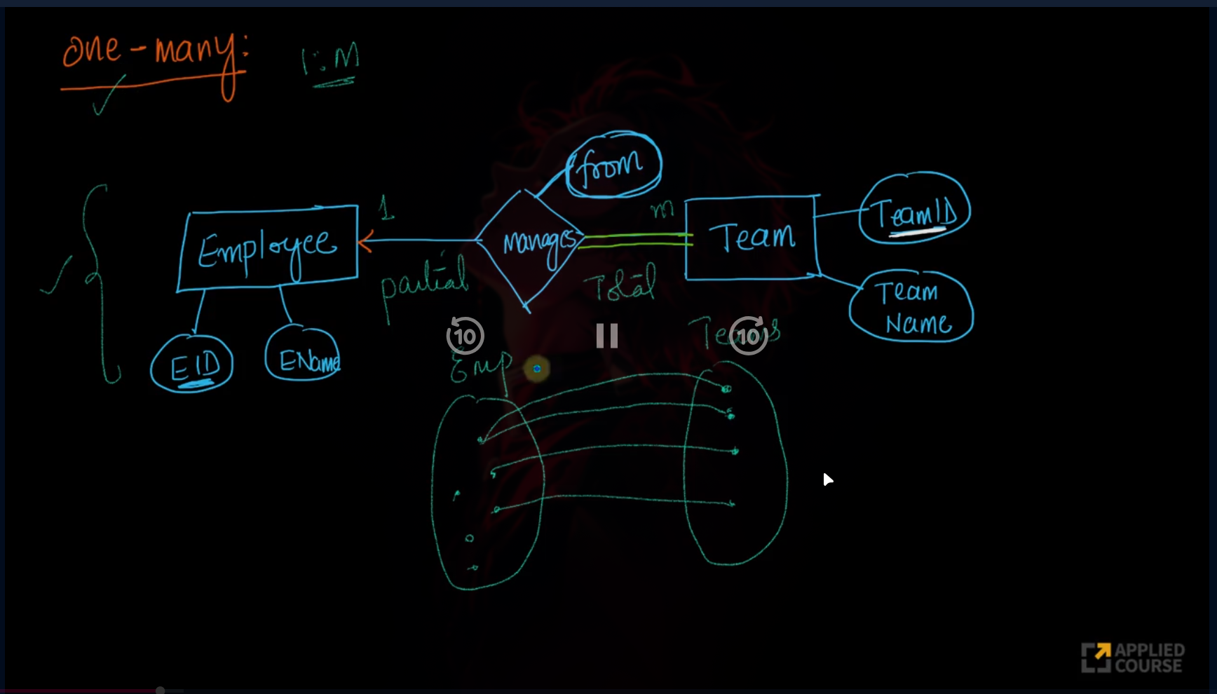
Relationships

Association among two or more entities.

Types:

• Strong Relationship: Between two independent entities
• Weak Relationship: Between weak entity and its owner/strong entity

Degree of Relationship:

• Unary: Only one entity participates
• Binary: Two entities participate
• Ternary: Three entities participate

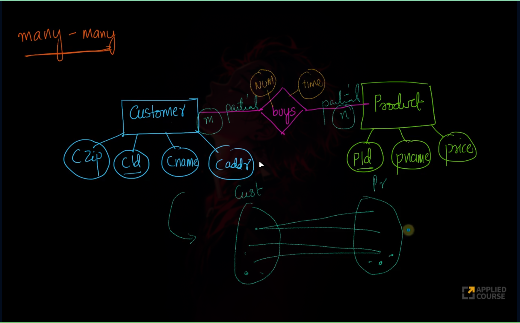
Relationship Cardinalities

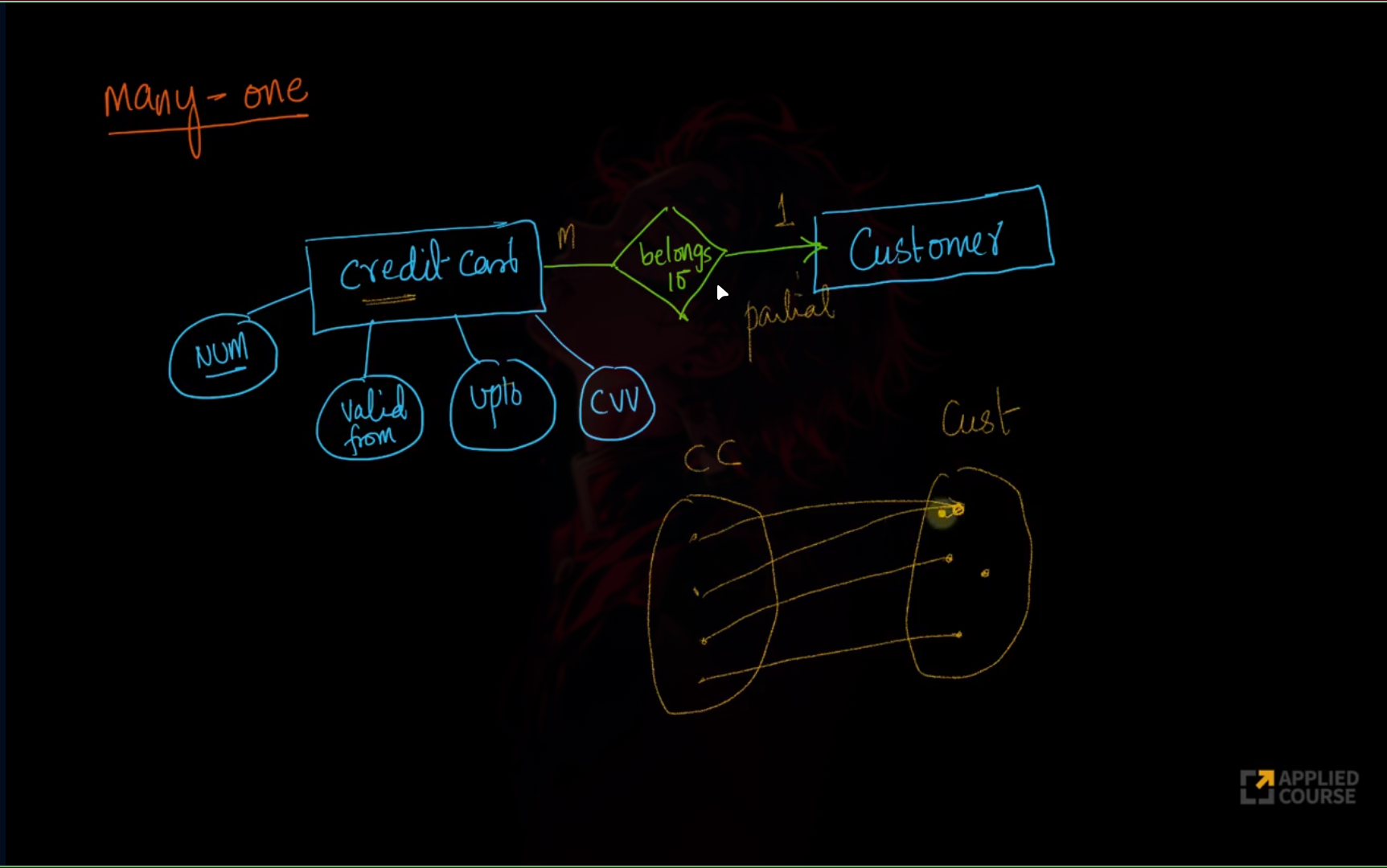
Strong vs Weak Entity

Strong Entity:

• Can be uniquely identified by its own attributes
• Has a primary key
• Shown with single rectangle in ER diagram

Weak Entity:

• Cannot be uniquely identified by its own attributes alone
• Depends on a strong entity (owner entity)
• Shown with double rectangle in ER diagram

---

Normalization

DBMS Normalization is a systematic approach to decompose tables to eliminate data redundancy. It is a multi-step process that puts data into tabular form, removes duplicate data, and sets up relationships between tables.

Why Normalization?

• Eliminating redundant data
• Keeping data consistent
• Storage optimization
• Making database structure more scalable and adaptable

Problems Without Normalization

If a table is not properly normalized and has data redundancy, it will:

• Consume extra memory
• Make it difficult to handle and update data
• Lead to Insertion, Update, and Deletion Anomalies

Example Table:

rollno	name	branch	hod	office_tel
401	Akon	CSE	Mr.X	123
402	Bkon	CSE	Mr.X	123
403	Ckon	CSE	Mr.X	123
404	Dkon	CSE	Mr.X	123

Insertion Anomaly

• Until a student opts for a branch, data cannot be inserted
• Branch information repeated for all students

Update Anomaly

• If HOD changes, all student records must be updated
• Risk of data inconsistency if some records are missed

Deletion Anomaly

• Deleting the last student in a branch loses branch information
• Two different entities (Student and Branch) should not be kept together

Normal Forms

First Normal Form (1NF)

Rules:

• Should only have single (atomic) valued attributes/columns
• All columns should have unique names

Example:

Not in 1NF:

StudentID	Name	Subjects
1	Raj	Math, Physics
2	Roy	Chemistry, Biology

In 1NF:

StudentID	Name	Subject
1	Raj	Math
1	Raj	Physics
2	Roy	Chemistry
2	Roy	Biology

Second Normal Form (2NF)

Rules:

• Must be in 1NF
• Should not have partial dependencies

Partial Dependency: When a non-prime attribute depends on part of a composite primary key.

Example:

Not in 2NF:

StudentID	SubjectID	StudentName	SubjectName
1	101	Raj	Math
1	102	Raj	Physics

In 2NF (split into 3 tables):

Students:

StudentID	StudentName
1	Raj
2	Roy

Subjects:

SubjectID	SubjectName
101	Math
102	Physics

Enrollments:

StudentID	SubjectID
1	101
1	102

Third Normal Form (3NF)

Rules:

• Must be in 2NF
• No transitive dependency

Transitive Dependency: When a non-prime attribute depends on another non-prime attribute.

Example:

Not in 3NF:

EmployeeID	EmployeeName	DeptID	DeptName	DeptLocation
1	Aman	10	IT	Mumbai
2	Neha	20	HR	Delhi

In 3NF:

Employees:

EmployeeID	EmployeeName	DeptID
1	Aman	10
2	Neha	20

Departments:

DeptID	DeptName	DeptLocation
10	IT	Mumbai
20	HR	Delhi

Boyce-Codd Normal Form (BCNF)

Rules:

• Must be in 3NF
• For each functional dependency (X → Y), X should be a Super Key

Example:

Not in BCNF:

studentId	Course	Instructor
1	DBMS	Raj
2	DS	Raj
3	AI	Roy

In BCNF:

Courses:

Course	Instructor
DBMS	Raj
DS	Raj
AI	Roy

Student Courses:

studentId	Course
1	DBMS
2	DS
3	AI

Fourth Normal Form (4NF)

Rules:

• Must be in BCNF
• No multi-valued dependency

Example:

Not in 4NF:

Student	Course	Hobby
Raj	DBMS	Cricket
Raj	DBMS	Music
Raj	AI	Cricket
Raj	AI	Music

In 4NF:

Student Courses:

Student	Course
Raj	DBMS
Raj	AI

Student Hobbies:

Student	Hobby
Raj	Cricket
Raj	Music

Fifth Normal Form (5NF)

Rules:

• Must be in 4NF
• Also called Project-Join Normal Form (PJNF)
• Most advanced level of normalization
• Cannot be decomposed without losing data

Example:

Not in 5NF:

Supplier	Part	Project
S1	P1	J1
S1	P1	J2
S1	P2	J1
S1	P2	J2

In 5NF:

Supplier Parts:

Supplier	Part
S1	P1
S1	P2

Supplier Projects:

Supplier	Project
S1	J1
S1	J2

Part Projects:

Part	Project
P1	J1
P1	J2
P2	J1
P2	J2

Advantages of Normalization

• Reduced data redundancy
• Improved data consistency
• Simplified database design
• Improved query performance
• Easier database maintenance

When to Use Normalization vs Denormalization

Normalization is best for:

• Transactional systems (banking, enterprise apps)
• Where data integrity is paramount

Denormalization is ideal for:

• Read-heavy applications
• Data warehousing
• Reporting systems
• Where performance is more critical than integrity

---

Transactions & Concurrency Control

A transaction is a sequence of one or more operations performed on the database as a single logical unit of work. It ensures that either all operations are successfully executed (committed) or none of them take effect (rolled back).

ACID Properties

Atomicity

• Transaction is all or nothing
• If any part fails, entire transaction is rolled back
• Example: Money transfer - both debit and credit must succeed

Consistency

• Transaction must keep database in valid state
• All constraints must hold
• Moves from one consistent state to another

Isolation

• Transactions run independently
• One transaction's operations should not affect another's
• Example: Two users withdrawing from same account

Durability

• Once committed, changes are permanent
• Survive system crashes
• Example: Updated balance remains after power failure

Transaction Schedules

Serial Schedule:

• Transactions execute one at a time
• Ensures consistency but reduces throughput

Non-Serial Schedule:

• Multiple transactions execute concurrently
• Interleaving operations
• Improves efficiency but requires concurrency control

Concurrency Control

Ensures consistency and integrity when multiple transactions execute simultaneously. Main goal is to prevent:

• Dirty Read: Reading uncommitted data
• Lost Update: Two transactions overwrite each other's changes
• Unrepeatable Read: Same query returns different values
• Phantom Read: New rows appear in repeated queries

DBMS uses locks, timestamps, and isolation levels to prevent these issues.

---

Indexing in DBMS

Disk Structure

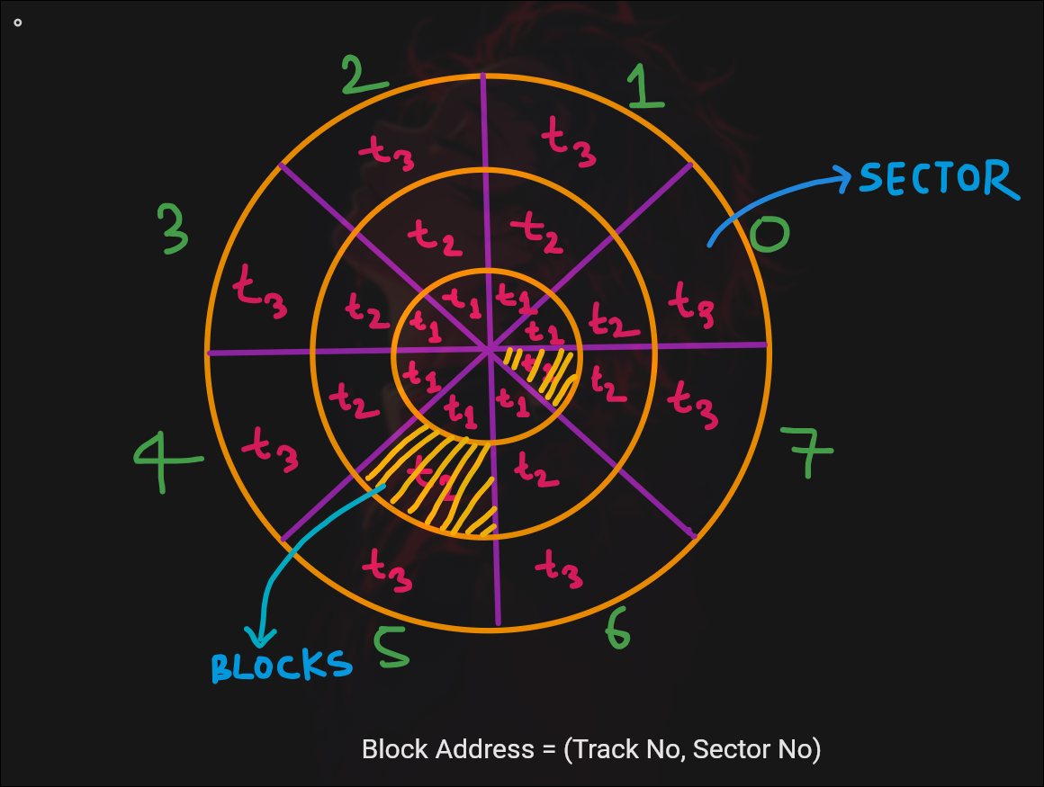
• Each block typically 512B
• Multiple rows stored per block
• Index table reduces search blocks needed

Index Benefits

Without indexing:

• Need to scan all data blocks
• Example: 100 records, 4 per block = 25 blocks to search

With indexing:

• Index table stores key-value pairs
• Key = ID, Value = pointer to block
• Drastically reduces search time

B-Trees

B-Tree is a specialized m-way tree designed for disk-based storage systems.

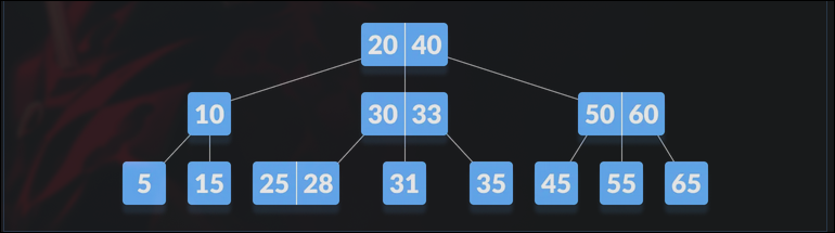
Properties:

• All leaf nodes at same level
• Keys stored in ascending order
• Non-leaf nodes (except root) have at least m/2 children
• Keys inserted bottom-up

Height formulas:

• Minimum height: ⌈log_m(n+1)⌉ - 1
• Maximum height: ⌈log_t(n+1)⌉

B+ Trees

Advanced version where:

• All data stored in leaf nodes
• Internal nodes contain only keys for navigation
• Leaf nodes are linked together
• Supports efficient range queries

BST vs B-Tree

BST:

• Each node has at most 2 children
• O(log n) if balanced, O(n) if skewed
• Stored in memory (RAM)

B-Tree:

• Many keys per node
• Fewer disk I/O operations
• Always balanced
• Optimized for databases

B-Tree vs B+ Tree

Feature	B-Tree	B+ Tree
Data Storage	Internal + leaf nodes	Leaf nodes only
Search Efficiency	May stop at internal nodes	Always goes to leaf
Range Queries	Needs in-order traversal	Fast (linked leaves)
Space Usage	Larger height	Smaller height
Use Case	General purpose	DBMS, file systems

Types of Indexing

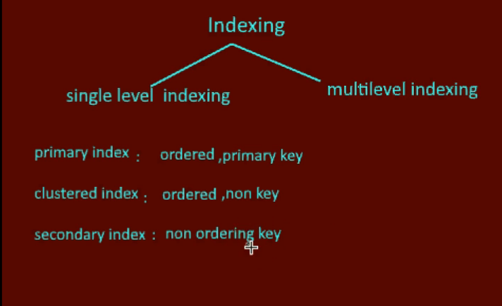
Primary Index

• Built on primary key
• Ordered index
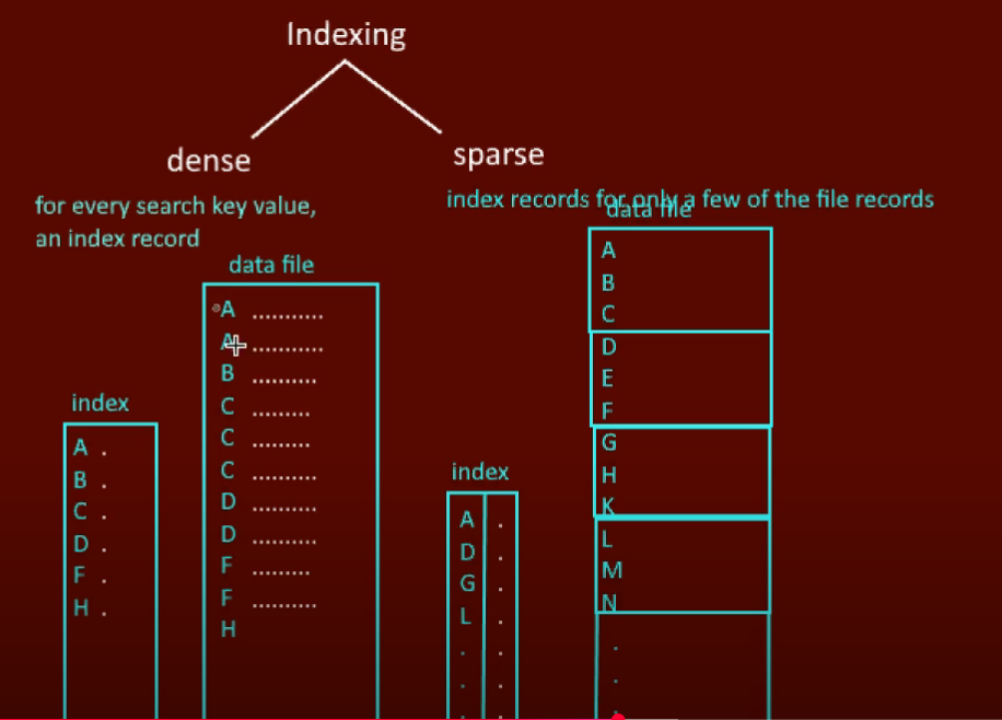
• Can be dense or sparse

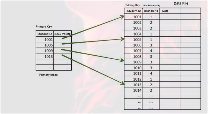
Dense Primary Index:

• Entry for every record
• Fast search but large size

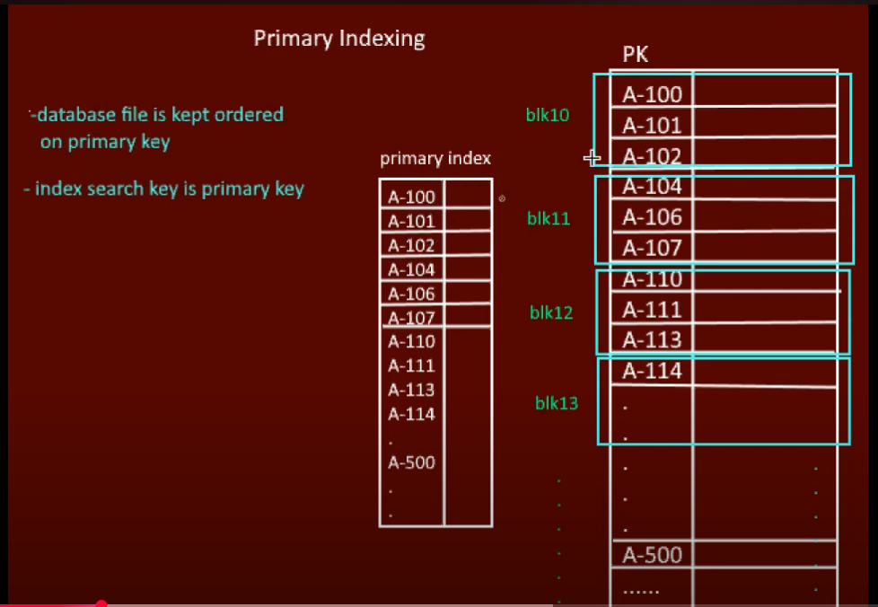
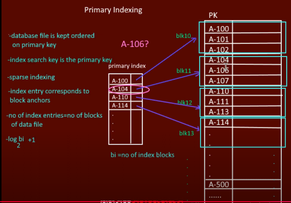
Sparse Primary Index:

• One entry per block
• Smaller index, slightly slower

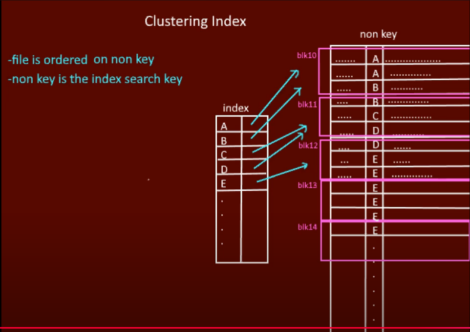
Clustering Index

• Built on non-primary key field
• Records physically grouped by clustering field
• One entry per distinct value

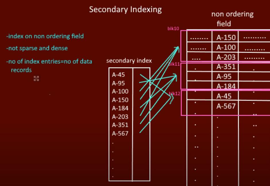
Secondary Index

• Built on non-clustering field
• Data file can be unordered
• Dense index (entry for every record)
• Multiple secondary indexes allowed

Dense vs Sparse Index

Feature	Dense Index	Sparse Index
Entries	One per record	One per block
Space	High	Low
Search	Very fast	Slower
Maintenance	Costly	Easier

Single Level vs Multilevel Indexing

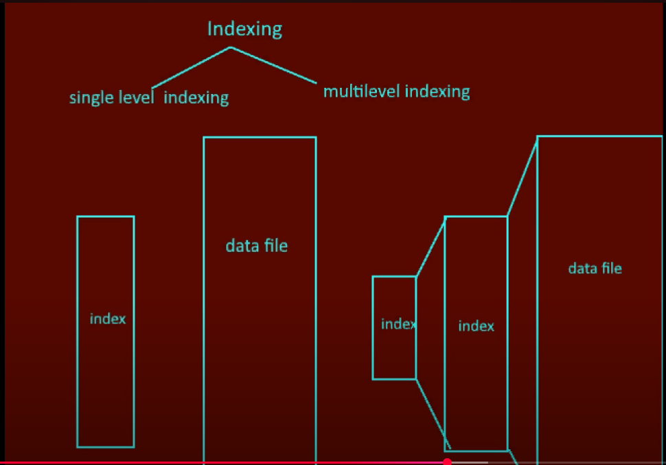
Single Level:

• One index file
• Slower for large data

Multilevel:

• Indexes on indexes
• Hierarchical structure (like B-Tree)
• Much faster for large databases

Index Types Summary

Index Type	Key Field	Record Order	Multiple Allowed
Primary	Primary Key	Sorted	No
Secondary	Non-Primary	Unsorted	Yes
Clustered	Any (usually PK)	Sorted	No
Non-Clustered	Any	Unsorted	Yes

---

NoSQL Databases

NoSQL stands for "Not Only SQL". Designed for:

• Unstructured/semi-structured data
• High scalability and availability
• Schema-less flexibility
• Distributed architecture

Key Characteristics

• Schema-free: No predefined structure
• Non-tabular: Uses JSON, key-value, etc.
• Handles big data: High volume and velocity
• Horizontal scaling: Distribute across servers
• Cloud-friendly: Built for cloud-native apps

Advantages

Flexible Schema

• No fixed schema required
• Easy to adapt to changes

Horizontal Scaling

• Add more servers to handle load
• Achieved via sharding or replica sets

High Availability

• Auto-replication across servers
• System continues if nodes fail

Fast Reads & Writes

• No joins needed
• Ideal for real-time apps

Built-in Caching

• Some NoSQL DBs (like Redis) serve as in-memory caches

When to Use NoSQL

• Fast-paced Agile development
• Unstructured/semi-structured data
• Huge data volumes
• Scalable architecture needed
• Real-time streaming, IoT, microservices

Types of NoSQL Databases

Key-Value Store

• Simplest type: key-value pairs
• Examples: Redis, DynamoDB
• Use: Caching, session management

Document Store

• Stores JSON-like documents
• Flexible schema
• Examples: MongoDB, CouchDB
• Use: E-commerce, CMS, mobile apps

Column-Oriented Store

• Stores data in columns
• Efficient for analytics
• Examples: Cassandra, HBase
• Use: Time-series, IoT, analytics

Graph Store

• Nodes and edges for relationships
• Examples: Neo4j, Amazon Neptune
• Use: Social networks, fraud detection

Disadvantages

• Data redundancy
• Costly deletes/updates
• Not one-size-fits-all
• Limited ACID support (varies)
• Lacks constraint enforcement

SQL vs NoSQL

Feature	SQL	NoSQL
Data Model	Tables	JSON, key-value, graphs
Schema	Fixed	Flexible
Scaling	Vertical	Horizontal
ACID	Full support	Partial
JOINs	Supported	Not needed
Examples	MySQL, PostgreSQL	MongoDB, Redis, Cassandra

---

Database Types

1. Relational Databases (RDBMS)

• Based on Relational Model
• Data in tables with rows and columns
• Use SQL
• ACID properties
• Examples: MySQL, PostgreSQL, Oracle

2. Object-Oriented Databases

• Based on OOP concepts
• Data as objects with methods
• Examples: ObjectDB, db4o
• Use: CAD/CAM, scientific apps

3. Hierarchical Databases

• Tree-like structure
• Parent-child relationships
• One-to-many only
• Examples: IBM IMS
• Use: File systems, XML

4. Network Databases

• Graph structure
• Many-to-many relationships
• Examples: IDMS
• Use: Telecom, engineering

---

Clustering in DBMS

Clustering connects multiple servers to manage a single database system.

Benefits

Data Redundancy

• Each node has data replica
• Prevents data loss

Load Balancing

• Requests distributed across servers
• No single machine overloaded

High Availability

• System remains available if nodes fail
• Critical for mission-critical systems

Scalability

• Easily add new nodes

Fault Tolerance

• Other servers continue if one fails

Architecture

Load Balancer
  ├── Node 1 (DB)
  ├── Node 2 (DB)
  └── Node 3 (DB)

---

Partitioning & Sharding

Partitioning

Splitting a large table into smaller, manageable parts.

Vertical Partitioning

• Divides by columns
• Each partition stores subset of attributes

Horizontal Partitioning

• Divides by rows
• Each partition contains different rows

When to Use

• Dataset too large
• Slow query response
• Multiple concurrent requests

Benefits

Feature	Benefit
Parallelism	Multiple queries on different partitions
Availability	If one fails, others online
Performance	Smaller tables, faster indexes
Manageability	Easier backup/archival

Sharding

Special form of horizontal partitioning where each shard is on a separate database server.

Example:

• Users 1-1M → Shard 1
• Users 1M-2M → Shard 2

Advantages

• Scalability
• Availability
• Performance

Disadvantages

• Complexity
• Data skew
• Re-sharding difficulty
• Analytical queries harder

Scatter-Gather Problem

Query must search all shards even if few records match.

SELECT * FROM users WHERE email LIKE '%@gmail.com';

Results:

• High network traffic
• Increased query time
• CPU usage on all shards

---

CAP Theorem

Distributed system can guarantee only two of three:

• C – Consistency: All nodes see same data
• A – Availability: Every request gets response
• P – Partition Tolerance: System works despite network failures

CAP Trade-Offs

Model	Guarantees	Sacrifices	Example	Use Case
CP	Consistency + Partition	Availability	MongoDB	Banking
AP	Availability + Partition	Consistency	Cassandra	Social apps
CA	Consistency + Availability	Partition	MySQL	Enterprise

Note: Partition Tolerance is essential in distributed systems, so real choice is between Consistency and Availability.

---

Master-Slave Architecture

• Master DB: Handles all writes
• Slave DBs: Handle reads (replicas)

How It Works

• Writes go to master
• Reads served from slaves
• Replication: Synchronous or Asynchronous

CQRS Pattern

• Command (Write): Master
• Query (Read): Slaves

Advantages

• Scalability
• High availability
• Load balancing
• Data safety
• Performance

Challenges

• Replication lag
• Write bottleneck
• Complex configuration

---

Scaling Patterns (Case Study)

Pattern 1: Query Optimization

• Use indexes
• Caching (Redis)
• Connection pooling

Pattern 2: Vertical Scaling

• Upgrade hardware
• More RAM/CPU

Pattern 3: CQRS

• Read replicas
• Separate read/write

Pattern 4: Multi-Primary

• Distribute writes
• Logical ring replication

Pattern 5: Functional Partitioning

• Split by functionality
• User DB, Trip DB, etc.

Pattern 6: Sharding

• Horizontal scaling
• 50+ machines
• Region-based

Pattern 7: Data Center Partitioning

• Multiple global data centers
• Geo-routing
• Cross-DC replication

---

Summary

This comprehensive guide covers:

Database Fundamentals

• ER diagrams and relationships
• Normalization (1NF through 5NF)
• Keys and constraints
• Database architecture

Indexing

• B-Trees and B+ Trees
• Primary, secondary, clustered indexes
• Dense and sparse indexing

Transactions

• ACID properties
• Concurrency control
• Transaction schedules

Advanced Topics

• NoSQL databases
• Clustering and partitioning
• CAP theorem
• Scaling patterns